In the conventional approach, application of the standard EnKF method on a problem like this (e.g. large dimensional state vector) can become computationally expensive during the updating. Therefore, it is necessary to find a way to reduce the computational cost. With the newly proposed technique, the data assimilation step is carried out for each local region around a particular grid block and most of the matrix computations (e.g. computation of Kalman gain etc.) are done in the local low-dimensional subspaces. This greatly helps in speeding up the computational process. Since the data assimilation is done locally, it is independent of the data assimilations in other local regions. The singular value decomposition (SVD) of the state vector in the local region is carried out to analyze the variation in the dynamics in the local region. The important variables in terms of their variations can be determined by analyzing the components of the singular vectors corresponding to different state variables in a particular local region. The components of the first singular vector corresponding to ρmolar1 (molar density of CO2), ρmolar10 (molar density of C6), pressure, and porosity in one of the local regions at 203 days is shown in Fig. 1. This local region happens to be on the edge of CO2 flood front at this time (203 days) and is partially swept by CO2. It can be observed that the components of the first singular vector show large variations for CO2 and C6 which suggest that these state variables are important in this local region and should be updated during the EnKF scheme. The components of the first singular vector corresponding to pressure and porosity also show some variation in this local region, but the variation is not as significant as that observed in case of CO2 or C6. This might be the indication of the fact that, in this region, state variables like CO2 and C6 are more important than pressure or porosity. Therefore, we believe that the proposed localization scheme helps identify the important variables from the local neighborhood.

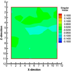
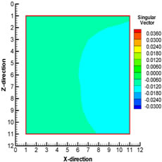
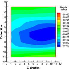
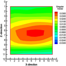
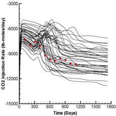
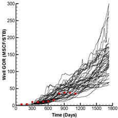
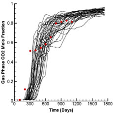
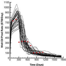
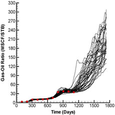
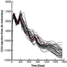
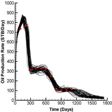
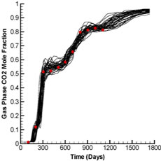
Fig. 2 shows the production and injection data obtained from the forward run of the initial ensemble (black lines) and the reference case (red dots) whereas